Stochastic parametersation of mesoscale wind kinetic energy

This is part of my PhD chapter where we investigated on a generalized approach to parameterise the commonly under-represented mesoscale wind variability in the re-analysis atmosphere field (e.g. ERA5). The atmosphere reanalysis data are commonly used to force a ocean simulations with realistic configuration. The wind forcing is the primary momentum input into the ocean that drives the large-scale general ocean circulation in the model. It is previsouly recognised that the presence of polar lows, tip jets associated with the orograhpic feature at the atmosphere-ocean boundry layer can change the modelled behavior of meridional overturning circulation (Condron and Renfrew, 2013), Pickart et al., 2003). These specific atmosphere phenomena were poorly resolved in reanalysis products due to the lack of resolution, but largely well-resolved now. In the meantime, the wind kinetic energy is still generally under-represented on a broad wavelength scales in the most recent ERA5 reanalysis wind field (Figure 1) even though the mesoscale wind systems (e.g., polar lows) are properly resolved.

We developed a generalized approach to parameterise ‘broadband’ wind energy deficiency over the mesoscale range on spatial and temporal domain (Figure 1), and we managed to rectify the wind kinentic energy spectra on the wavenumber and frequency domain at the same time (Figure 1). The parameterisation possesses folllowing advantages:

1. A direct control on the energetic characteristics of the parameterised wind field on wavenumber and frequency domain.
2. Easy to implement for attribution study in atmosphere-ocean coupling scheme.
3. Overall ‘correction’ or offset brought by the parameterisation on the mean state is small enough to be assessed and compared with the original ERA5 data.

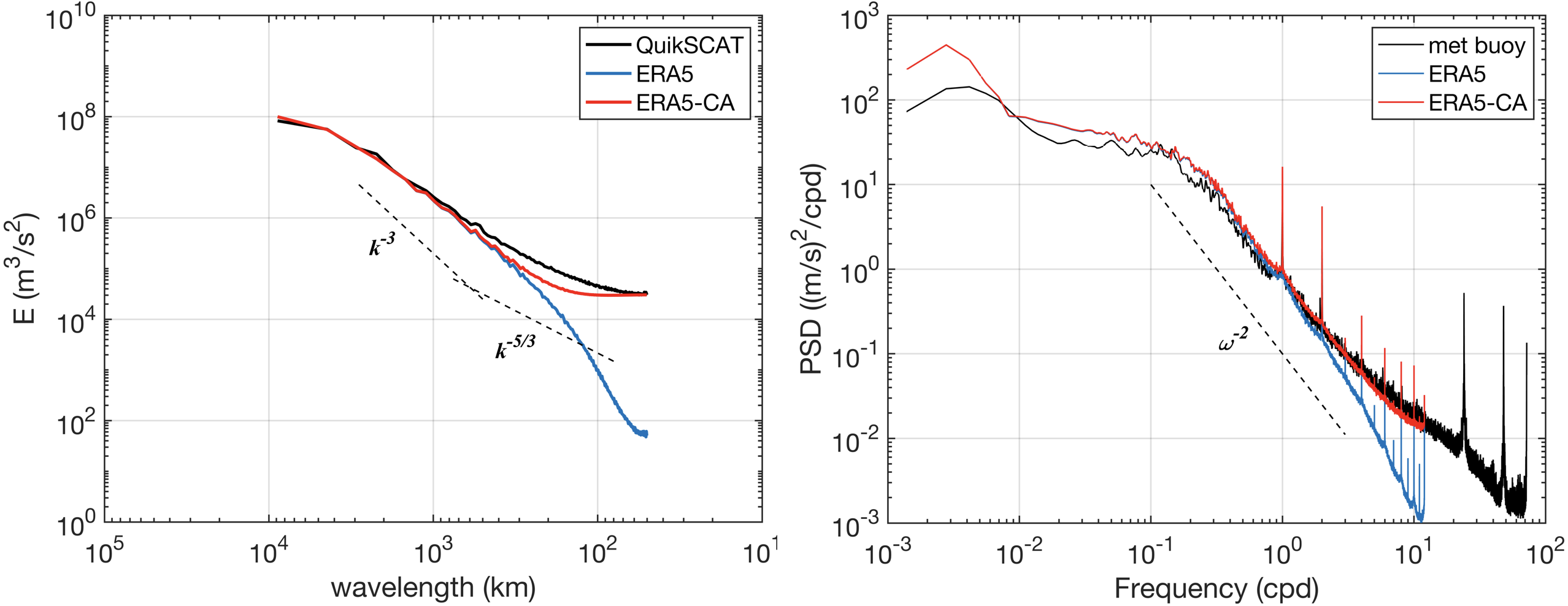Figure 1. (left) Wavenumber spectra of observation (QuikSCAT, black), reanalysis (ERA5, blue) and perturbed (red) wind field. (right) Same as the one on the left, but for the frequency domain.

The difference in the air-sea fluxes brought by the parameterisation of the wind variability is self-organized - wind enhancement over tropical and subtropical region, enhancement of wind stress curl in the subpolar and trade wind bands, and enhanced surface cooling in tropical and subtropical region. These changes in the surface fluxes lead to pronounced sea surface response where SST cooled significantly in the tropical and subtropical regions and the mixed layer depth deepened significantly in the subpolar region. Further changes from the surface forcing are translated into the systematic response of the general circulation simulated, such as the Atlantic Meridional Overturning Circulation (AMOC) and Subpolar Gyre (SPG).

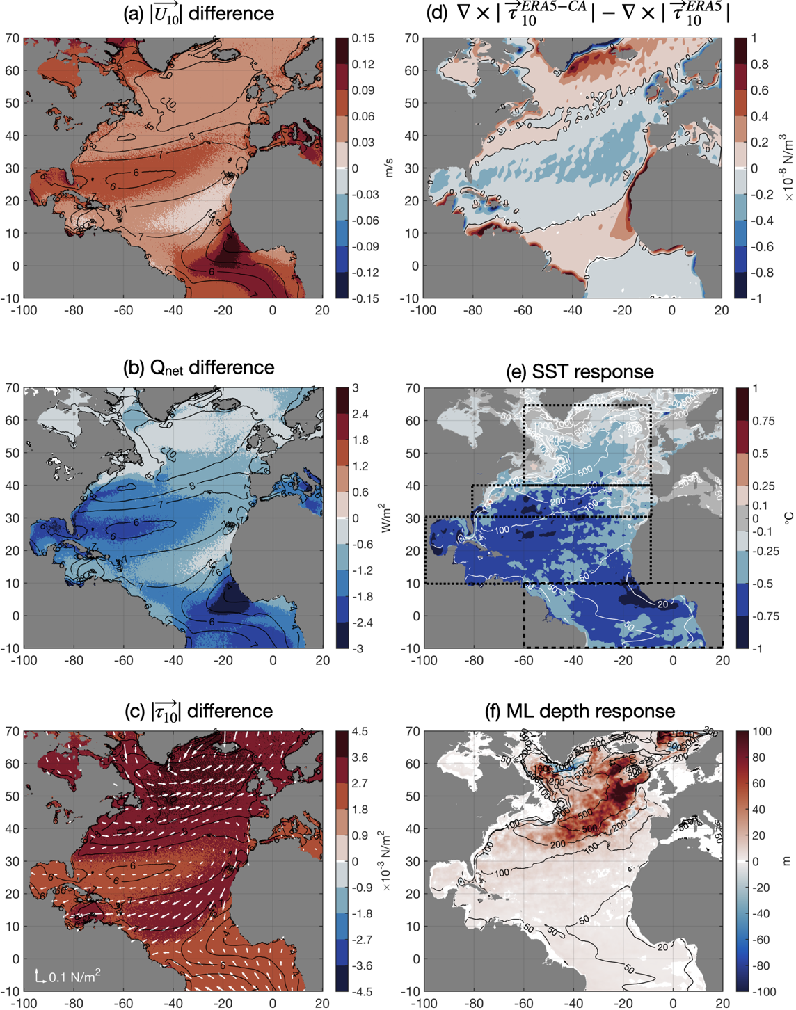Figure 2. Changes induced by the wind perturbations in the surface wind speed (\(|U_{10}|\)), net surface heat fluxes (\(Q_{net}\)), wind stress magnitude (\(|\tau_{10}|\)), wind stress curl (\(\nabla\times\tau_{10}\)), SST response and ML depth response.

The model captures a clear strengthening of the AMOC and SPG, accompanied by the enhanced northward heat transport in the upper 1000 m (Figure 3). The results suggest that the missing of the coherent spatio-temporal scales can still lead to a significantly different ocean circulation behavior. This may be of importance for the high-resolution ocean simulation of the AMOC and calls for careful treatment of the air-sea fluxes in these models considering the high sensitivity of the high-resolution ocean model to the subtle changes in the air-sea fluxes in critical regions. More can be found here.

Figure 3. (top) SPG transport simulated in control (black line) and perturbed ensembles (coloured lines) and the difference between ensemble members and the control (coloured bars) and the mean difference between ensemble and control simulation (broken black line). (middle) same as the top panel but for AMOC transport. (bottom) The difference between each ensemble member and control similation (coloured bars) and the mean difference between ensemble and control (broken black line) in the top 1000 m heat transport across 26°N, red curve denotes the cumulative heat transport difference across 26°N over the upper 1000 m.